Accueil > Linux / Logiciels Libres > Scilab > Modèle 3D dans Scilab
 Modèle 3D dans Scilab
dimanche 9 janvier 2011, par
Ces travaux ont fait l’objet de 2 publications dans la revue Linux Pratique :
Afficher des patchs dans Scilab
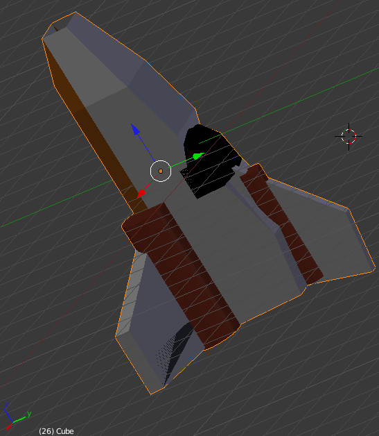
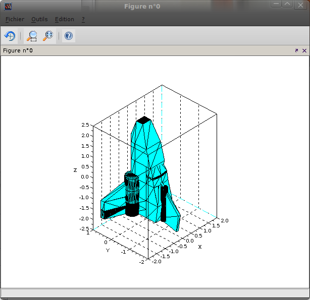
A partir de l’export 3DS d’un modème 3D blender, il est possible de réaliser un modèle 3D pour Scilab : un patch.
Le programme 3ds2mat suivant, basé sur la lib3ds. Il est prévu pour être compilé en « static » afin d’éviter les pbs de dépendances.
Après avoir téléchargée, désarchivée et compilée (sans l’installer) la « lib3ds », l’archive suivante doit être décompressée dans le répertoire « examples » de l’arborescence de la librairie « lib3ds ».
| Archive du programme |
|---|

Programme 3ds2mat
|
Lancez ensuite la compilation du programme 3ds2mat par « ./configure && make ».
Conversion d’un fichier 3DS en patch pour Scilab
Utilisez l’archive des modèles 3D suivante :
| Archive des modèles |
|---|
|
Modeles 3D et patchs
|
Le programme s’utilise comme suit :
./3ds2mat -t bsg_lowpoly.3ds > bsg_lowpoly.scel’affichage dans Scilab est réaliser à l’aide du code suivant :
//loads the 3D patch (a lowpoly one)
// from http://e2-productions.com/repository/modules/PDdownloads/viewcat.php?cid=17
exec('bsg_lowpoly.sce'); //exec('snowspeeder_scilab.sce');

//the face numbering starts à 1 (not 0 given by lib3ds)
facelist1 = facelist1 + 1;
// The face list indicates which points are composing the patch.

//some scaling to adjust the size of the patch to the model
scale_factor = 0.6;
vertices1 = vertices1 * scale_factor;

// The formula used to translate the vertex / face representation into x, y, z lists

xvf = matrix(vertices1(facelist1,1),size(facelist1,1),length(vertices1(facelist1,1))/size(facelist1,1))';
yvf = matrix(vertices1(facelist1,2),size(facelist1,1),length(vertices1(facelist1,1))/size(facelist1,1))';
zvf = matrix(vertices1(facelist1,3),size(facelist1,1),length(vertices1(facelist1,1))/size(facelist1,1))';
//plot the patch in 3D
plot3d(xvf,yvf,zvf,flag=[1,4,4]);
set(gca(),"grid",[1 1]);
On obtient :
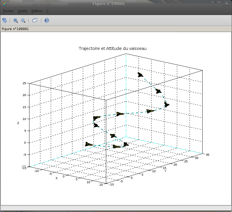
Mise en situation des patchs 3D sur une trajectoire
//3D trajectory
t=0:0.01:10;
x=10*sin(t);
y=3*t;
z=0.2*t.^2;
//loads the 3D patch (a lowpoly one)
// from http://e2-productions.com/repository/modules/PDdownloads/viewcat.php?cid=17
exec('bsg_lowpoly.sce');
//exec('snowspeeder_scilab.sce');
//the face numbering starts à 1 (not 0 given by lib3ds)
facelist1 = facelist1 + 1;
// The face list indicates which points are composing the patch.
//some scaling to adjust the size of the patch to the model
scale_factor = 0.3;
vertices1 = vertices1 * scale_factor;
// The formula used to translate the vertex / face representation into x, y, z lists
xvf = matrix(vertices1(facelist1,1),size(facelist1,1),length(vertices1(facelist1,1))/size(facelist1,1))';
yvf = matrix(vertices1(facelist1,2),size(facelist1,1),length(vertices1(facelist1,1))/size(facelist1,1))';
zvf = matrix(vertices1(facelist1,3),size(facelist1,1),length(vertices1(facelist1,1))/size(facelist1,1))';
//orienting the patch on the curve (tangent)
dx = diff(x);
dy = diff(y);
dz = diff(z);
// from http://fr.wikipedia.org/wiki/Coordonn%C3%A9es_sph%C3%A9riques
// and from http://jeux.developpez.com/faq/math/?page=transformations#Q31
// the next line computes theta_v according to y > 0 or < 0
//((bool2s(dy > 0)*2) -1) .* acos(dx./(sqrt(dx.^2+dy.^2))) + bool2s(dy < 0)*2*%pi;
rho_v = sqrt(dx.^2+dy.^2+dz.^2); //distance computing
phi_v = acos(dz./rho_v); //X Axis Rotation pitch
theta_v = ((bool2s(dy > 0)*2) -1).*acos(dx./(sqrt(dx.^2+dy.^2))) + bool2s(dy < 0)*2*%pi;
theta_v = - theta_v + %pi/2; //A rotation axis yaw
psi_v = [0];
psi_v = [ psi_v diff(theta_v)] *30; // roll
curFig = scf(100001);
clf(curFig,"reset");
curFig.axes_size = [ 1600 1200 ];
curFig.figure_position = [100,100]
//some adjustments due to blender and scilab
theta =theta_v(1); //tangage autour de l'axe vertical Y = yaw
phi = phi_v(1); //piqué rotation autour de X aile de l avion = pitch
psi = psi_v(1); //roulis autour de l'axe nez-queue = roll
//Definition of rotation matrix terms
A = cos(phi);
B = sin(phi);
C = cos(psi);
D = sin(psi);
E = cos(theta);
F = sin(theta);
//rotation matrix
M = [ C*E -C*F -D;
-B*D*E+A*F -B*D*F+A*E -B*C;
A*D*E+B*F -A*D*F+B*E A*C];
vertex_new=vertices1*M;
xvf = matrix(vertex_new(facelist1,1),size(facelist1,1),length(vertex_new(facelist1,1))/size(facelist1,1))';
yvf = matrix(vertex_new(facelist1,2),size(facelist1,1),length(vertex_new(facelist1,1))/size(facelist1,1))';
zvf = matrix(vertex_new(facelist1,3),size(facelist1,1),length(vertex_new(facelist1,1))/size(facelist1,1))';
//moving the patch on the curve
xvf = xvf + x(1);
yvf = yvf + y(1);
zvf = zvf + z(1);
alpha_view = 310; //initial angle
theta_view = 70; //initial angle
curAxe=gca();
curAxe.data_bounds=[-11 -6 -6; 11 32 22];
set(curAxe,"grid",[1 1 1]);
//plot the 3D trajectory
param3d(x,y,z,flag=[0,4]);
//plot the patch
plot3d(xvf,yvf,zvf,alpha_view,theta_view,flag=[1,0,4]);
//getting the handle on the 3D curve
line=curAxe.children(2); //second plot = curve
line.line_style=3; //define the line style
line.thickness=2; //define the thickness of the line
line.foreground=16; //define the color of the line
//line.polyline_style=3;
//getting the handle on the 3D patch
patch=curAxe.children(1); //first plot = patch
//line.line_style=3; //define the line style
patch.thickness=0.5; //define the thickness of the lines
patch.foreground=1; ////define the color of the lines
patch.color_mode=1; //define the color of the patch
patch.hiddencolor=7; //define the color of the patch
for i = 1:size(t,2)
if (modulo(i,100)==0) //allow to plot 1 every 100
//some adjustments due to blender and scilab
theta = theta_v(i);
phi = phi_v(i);
psi = psi_v(i); //no roll, but we can simulate it
//Definition of rotation matrix terms
A = cos(phi);
B = sin(phi);
C = cos(psi);
D = sin(psi);
E = cos(theta);
F = sin(theta);
M = [ C*E -C*F -D;
-B*D*E+A*F -B*D*F+A*E -B*C;
A*D*E+B*F -A*D*F+B*E A*C];
vertex_new=vertices1*M;
xvf = matrix(vertex_new(facelist1,1),size(facelist1,1),length(vertex_new(facelist1,1))/size(facelist1,1))';
yvf = matrix(vertex_new(facelist1,2),size(facelist1,1),length(vertex_new(facelist1,1))/size(facelist1,1))';
zvf = matrix(vertex_new(facelist1,3),size(facelist1,1),length(vertex_new(facelist1,1))/size(facelist1,1))';
//moving the patch on the curve
xvf = xvf + x(i);
yvf = yvf + y(i);
zvf = zvf + z(i);
plot3d(xvf,yvf,zvf,alpha_view,theta_view,flag=[1,0,4]);
//getting the handle on the 3D patch
patch=curAxe.children(1); //last plot = first children = patch
//line.line_style=3; //define the line style
patch.thickness=0.5; //define the thickness of the lines
patch.foreground=1; ////define the color of the lines
patch.color_mode=1; //define the color of the patch
patch.hiddencolor=7; //define the color of the patch
end;
end;
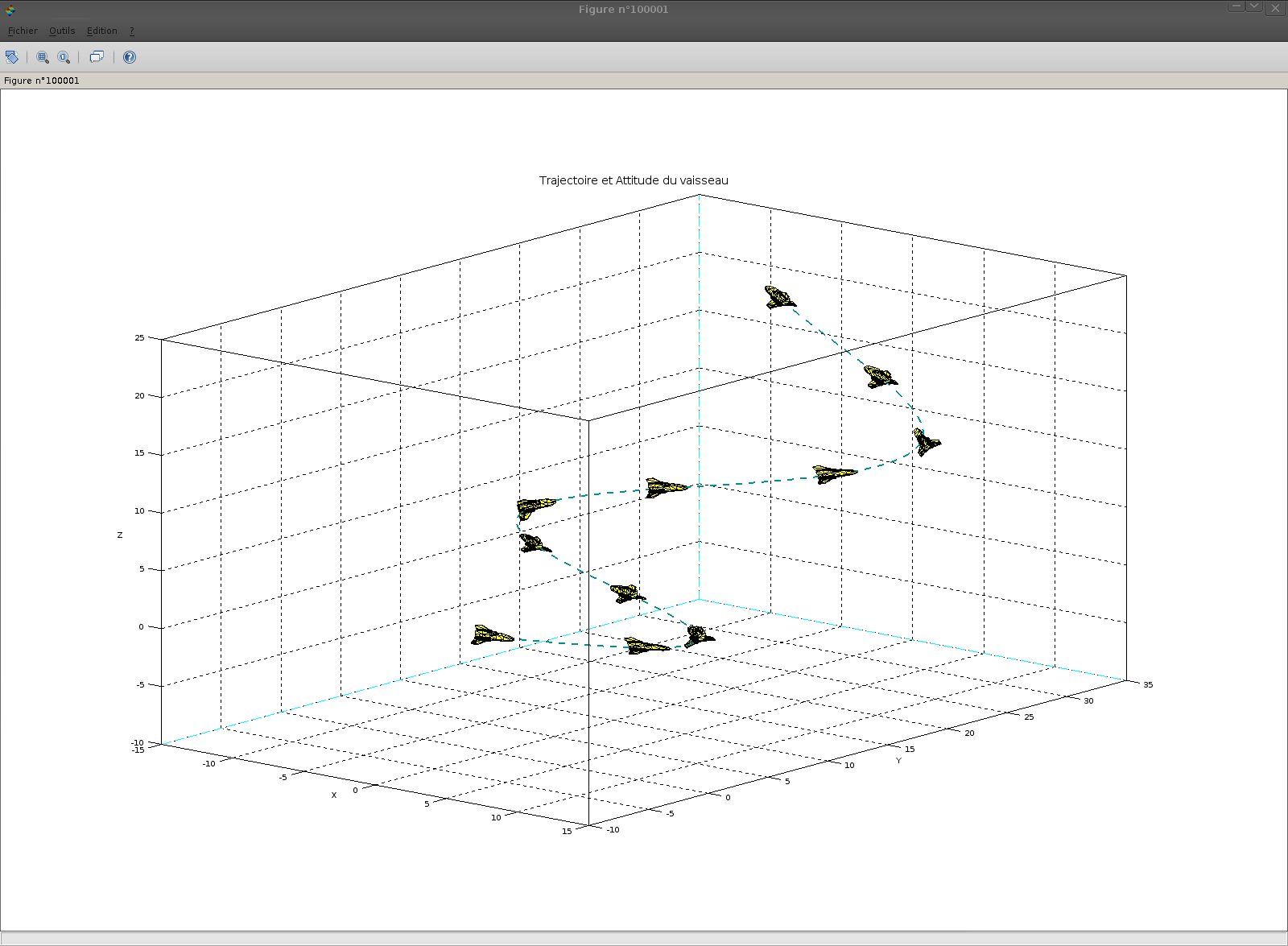
title("Trajectoire et Attitude du vaisseau","fontsize",3);donne :
Animation simple dans Scilab
realtimeinit(0.01);//sets time unit to half a second
realtime(0);//sets current date to 0

xinit(); //create a figure
a=get("current_axes");//get the handle of the newly created axes
a.data_bounds=[-%pi,-1.1;%pi,1.1]; //fix the bounds
a.grid=[1 1]; //create the 2D grid

x = -%pi:2*%pi/100:%pi; //create the data
y=sin(x); //create the data
y2=sin(4*x); //create the data

drawlater(); //we delay the plotting

// first plot to create all objects for future access
plot(x(1),y(1),'b',x(1),y2(1),'r'); //plot only needed data

curAxe=gca(); //get the current axe handle

sin1=curAxe.children(1).children(1); //get the handle on 1st sinus
sin2=curAxe.children(1).children(2); ////get the handle on 2nd sinus

for k=2:101
    sin1.data = [x(1:k)',y(1:k)']; //we only replace the data
    sin2.data = [x(1:k)',y2(1:k)']; ////we only replace the data
    realtime(k); //every wait time
    drawnow(); //plotting
end

realtimeinit(0.1);//sets time unit to half a second
realtime(0);//sets current date to 0

x= [0 0 1 1];
y = [0 1 1 0];

xinit(); //create a figure
curAxes = gca();
//curAxes.data_bounds=[-1,-1;2,2]; //fix the bounds
square(-1,-1,2,2);
curAxes.grid=[1 1]; //create the 2D grid

xset("color",2)
xfpoly(x,y);
drawlater();
xy = [x;y];
t = 0:2*%pi/100:2*%pi;
//rotation
for  i=1:length(t),
    drawlater();
    xy1=rotate(xy,t(i),[0.5;0.5]);
    curAxes.children(1).data = xy1';
    realtime(i); //every wait time
    drawnow();
end


drawlater();
//déplacement
realtimeinit(0.01);
realtime(0);
t = 0:2*%pi/100:2*%pi
//x_pos = sin(t);
x_pos = linspace(0,1, length(t));
y_pos = linspace(0,1, length(t));
//y_pos = cos(t);
for  i=1:length(t),
    drawlater();
    x_new = x +x_pos(i);
    y_new = y +y_pos(i);
    xy1 = [x_new;y_new];
    curAxes.children(1).data = xy1';
    realtime(i); //every wait time
    drawnow();
end

//les deux
drawlater();
//déplacement
realtimeinit(0.1);
realtime(0);
t = 0:2*%pi/100:2*%pi
x_pos = cos(t);
//x_pos = linspace(0,1, length(t));
//y_pos = linspace(0,1, length(t));
y_pos = sin(t);
for  i=1:length(t),
    drawlater();
    xy1=rotate(xy,4*t(i),[0.5;0.5]);
    x_new = xy1(1,:)+x_pos(i);
    y_new = xy1(2,:)+y_pos(i);
    curAxes.children(1).data = [x_new;y_new]';
    realtime(i); //every wait time
    drawnow();
end

Animation de notre vaisseau avec scilab et création d’un GIF animé
clear all;
usecanvas(%F);
//usecanvas(%F); si la carte graphique supporte et en met pas le warning
//ATTENTION : A cause des limitations de votre configuration, Scilab est passé dans un mode dans lequel mélanger des uicontrols et des graphique n'est pas possible. Tapez "help usecanvas" pour plus d'information
//Scilab uses a "GLJPanel" %F (a Swing OpenGL component) to display graphics (plot3d, plot, ...). This component uses some high level OpenGL primitives which are not correctly supported on some platforms (depending on the operating system, video cards, drivers ...)
//Linux
//NVIDIA Card With free drivers.
//ATI Card With free drivers or ATI-drivers with version < 8.52.3 (Installer version < 8.8 / OpenGL version < 2.1.7873).
// INTEL Card With Direct Rendering activated.
//Simulated 3D trajectory
t=0:0.1:10;
x=10*sin(t);
y=3*t;
z=0.2*t.^2;
//loads the 3D patch (a lowpoly one)
// from http://e2-productions.com/repository/modules/PDdownloads/viewcat.php?cid=17
exec('bsg_lowpoly.sce');
//exec('snowspeeder_scilab.sce');
//the face numbering starts à 1 (not 0 given by lib3ds)
facelist1 = facelist1 + 1;
// The face list indicates which points are composing the patch.
//some scaling to adjust the size of the patch to the model
scale_factor = 0.4;
vertices1 = vertices1 * scale_factor;
// The formula used to translate the vertex / face representation into x, y, z lists
xvf = matrix(vertices1(facelist1,1),size(facelist1,1),length(vertices1(facelist1,1))/size(facelist1,1))';
yvf = matrix(vertices1(facelist1,2),size(facelist1,1),length(vertices1(facelist1,1))/size(facelist1,1))';
zvf = matrix(vertices1(facelist1,3),size(facelist1,1),length(vertices1(facelist1,1))/size(facelist1,1))';
//orienting the patch on the curve (tangent)
dx = diff(x);
dy = diff(y);
dz = diff(z);
// from http://fr.wikipedia.org/wiki/Coordonn%C3%A9es_sph%C3%A9riques
// and from http://jeux.developpez.com/faq/math/?page=transformations#Q31
// the next line computes theta_v according to y > 0 or < 0
//((bool2s(dy > 0)*2) -1) .* acos(dx./(sqrt(dx.^2+dy.^2))) + bool2s(dy < 0)*2*%pi;
rho_v = sqrt(dx.^2+dy.^2+dz.^2); //distance computing
phi_v = acos(dz./rho_v); //X Axis Rotation : Pitch is acting about an axis perpendicular to the longitudinal plane of symmetry
theta_v = ((bool2s(dy > 0)*2) -1).*acos(dx./(sqrt(dx.^2+dy.^2))) + bool2s(dy < 0)*2*%pi;
theta_v = - theta_v + %pi/2; //A rotation axis yaw : The yaw is about the vertical body axis,
psi_v = [0];
psi_v = [ psi_v diff(theta_v)] *2; // roll is acting about the longitudinal axis
curFig = scf(100001);
clf(curFig,"reset");
curFig.axes_size = [ 1600 1200 ];
curFig.figure_position = [100,100]
//Set the evolution of the view angles Theta and Alpha
//---------------------------------------------------
alpha_view = 260; //initial angle
alpha_end_view = 245;//215; // final angle
theta_view =75; //initial angle
theta_end_view = 75; // final angle
A=linspace(alpha_view,alpha_end_view, size(t,2)-1);
T=linspace(theta_view,theta_end_view, size(t,2)-1);
Angles=[T;A]; //Angle Matrix
drawlater(); // delay the plotting until drawnow() is called
show_window(curFig); //raise the graphic window
//plot the 3D trajectory
param3d(x,y,z,flag=[0,4]);
curAxe=gca();
//plot the patch in "initial" position
plot3d(xvf,yvf,zvf,alpha_view,theta_view,flag=[1,0,4]);
set(gca(),"grid",[1 1 1]); //put the grid on the figure
// set 3D boundaries
curAxe.data_bounds=[-11 -6 -6; 11 32 22];
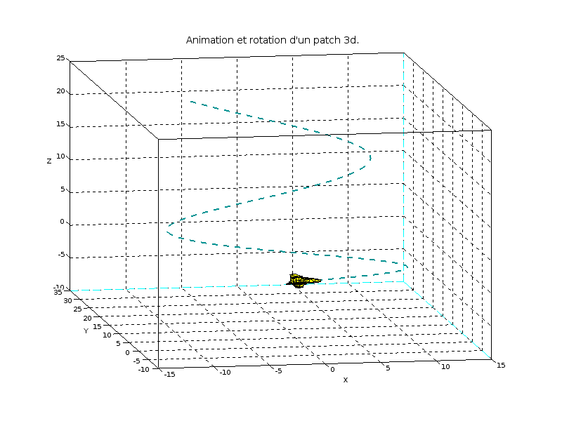
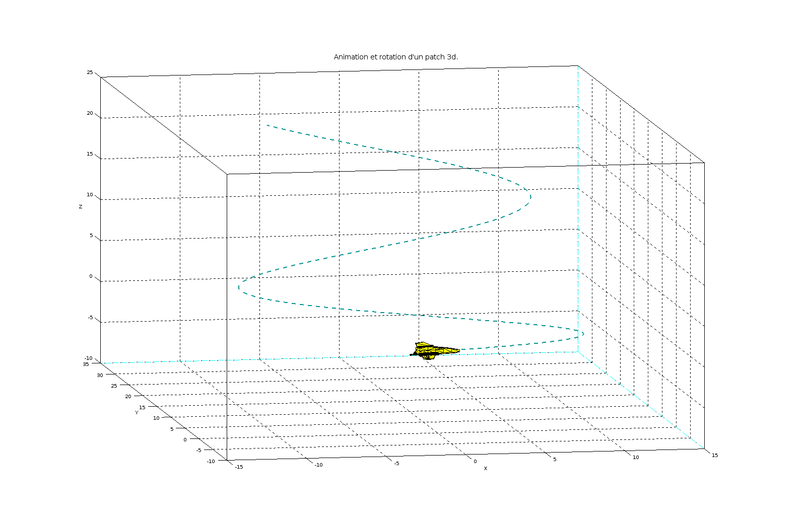
title("Animation et rotation d''un patch 3d.","fontsize",3);
s=gce(); //the handle on the surface
//curFig.background = -1; // black
//curAxe.background = -1; // gray
//curAxe.foreground = 14; // white
//getting the handle on the 3D curve
line=curAxe.children(2); //second plot = curve
line.line_style=3; //define the line style
line.thickness=2; //define the thickness of the line
line.foreground=16; //define the color of the line
//line.polyline_style=3;
//getting the handle on the 3D patch
patch=curAxe.children(1); //first plot = patch
//line.line_style=3; //define the line style
patch.thickness=0.5; //define the thickness of the lines
patch.foreground=1; ////define the color of the lines
patch.color_mode=1; //define the color of the patch
patch.hiddencolor=7; //define the color of the patch
winnum=winsid();//getting the window number
//drawnow();
frame_duration = 0.05
realtimeinit(frame_duration); //fix (if possible, regarding to calculus) the duration of one frame
realtime(0);
for i = 1:size(t,2)-1 //due to the the "diff" computing
drawlater();
//setting the angles
theta = theta_v(i); //Yaw
phi = phi_v(i); //Pitch
psi = psi_v(i); //Roll
//Definition of rotation matrix terms
A = cos(phi);
B = sin(phi);
C = cos(psi);
D = sin(psi);
E = cos(theta);
F = sin(theta);
//Definition of the rotationmatrix
M = [ C*E -C*F -D;
-B*D*E+A*F -B*D*F+A*E -B*C;
A*D*E+B*F -A*D*F+B*E A*C];
//new verteces locations
vertex_new=vertices1*M;
//modification of the patch on the figure
s.data.x = matrix(vertex_new(facelist1,1),size(facelist1,1),length(vertex_new(facelist1,1))/size(facelist1,1))' + x(i);
s.data.y = matrix(vertex_new(facelist1,2),size(facelist1,1),length(vertex_new(facelist1,1))/size(facelist1,1))' + y(i);
s.data.z = matrix(vertex_new(facelist1,3),size(facelist1,1),length(vertex_new(facelist1,1))/size(facelist1,1))' + z(i);
//if rotation animation
curAxe.rotation_angles = Angles(:,i); //change the view angles property
realtime(i); //wait till date frame_duration*i seconds
drawnow(); //plotting all the stuff on the figure
//recording each frame in a gif file (see doc for other format)
if pmodulo(i,1)==0 then //use pmodulo to save a frame each n frame
nom_image='capture/image_'+string(1000+i)+'.gif';
xs2gif(winnum,nom_image);//on sauve dans le répertoire courant
//create animated gif with imagemagic fabulous convert program :-)
//convert -delay 10 -loop 0 image2_*.gif animation2.gif
nom_image='capture/image_'+string(1000+i)+'.png';
xs2png(winnum,nom_image);//on sauve dans le répertoire courant
//create animated png with apngasm program :-)
//./apngasm output.png image_1*.png 1 10 /l0
end
endce qui donne en Gif

et en Png